What Is a Mesh? From LiDAR Points to 3D Files, Explained Simply

Take a LiDAR scan of a hill and a 3D model of the same hill. On screen they look almost the same. Now try opening both in Blender. The model loads fine. The scan won’t open at all, because Blender doesn’t read LAS files and wouldn’t know what to do with one anyway.

The gap between those two files is the whole subject of this post. One is a pile of measurements. The other is a surface. Getting from the first to the second is called meshing, and once you see what a mesh file actually contains, most of the jargon around it stops being scary.

The hill is a good example to carry through, so I’ll stick with it. The drawings use a simple hill with a drone flying over it. When we get to the code, we’ll switch to a real LiDAR scan of a real hill, Mount Tabor in Portland, and turn it into a 3D file we can measure, view in a browser and send to anyone.

Dots, not a surface

A LiDAR scanner fires laser pulses and times each echo. The time tells it the distance, and since the scanner also knows exactly where it is and which way it was pointing, every echo turns into one point in space: an x, a y and a z (the height).

A drone does this hundreds of thousands of times a second. What comes out is a point cloud, normally stored as a .las file (or .laz, the compressed version).

Viewed from a distance, a point cloud looks solid. Zoom in and it falls apart. There’s nothing between the dots, you can see through the hill to the far side, and the file has no idea which dots are neighbours. So you can’t ask it for the surface area, there’s nothing to shine a light on, and a 3D printer has no outline to print.

Connecting the dots

A mesh fixes that by joining nearby points into triangles. Lay enough triangles edge to edge and they cover the hill completely, a bit like a fishing net pulled tight over it.

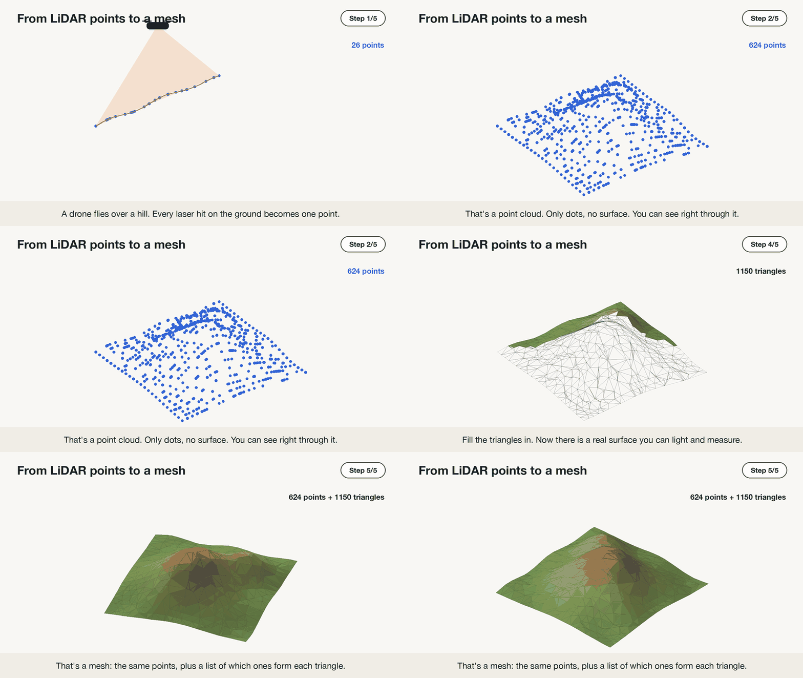624 points from start to finish. Nothing gets added except the triangles.

Notice the points never move. The mesh keeps every one of them and adds a second piece of information: which three points make up each triangle. In 3D-speak the points are vertices, the triangles are faces, and the line where two triangles meet is an edge.

Why triangles, and not squares? Think of a stool. A three-legged stool never wobbles, even on a bumpy floor, because three legs always touch the ground together. A four-legged chair can wobble, because one leg can end up higher than the others.

Shapes in a mesh work the same way. A triangle is always perfectly flat, wherever its three corners are. A square made from four scanned points often isn’t, because one corner can sit a little higher than the rest, and then the square bends in the middle. The computer has to guess where that bend goes.

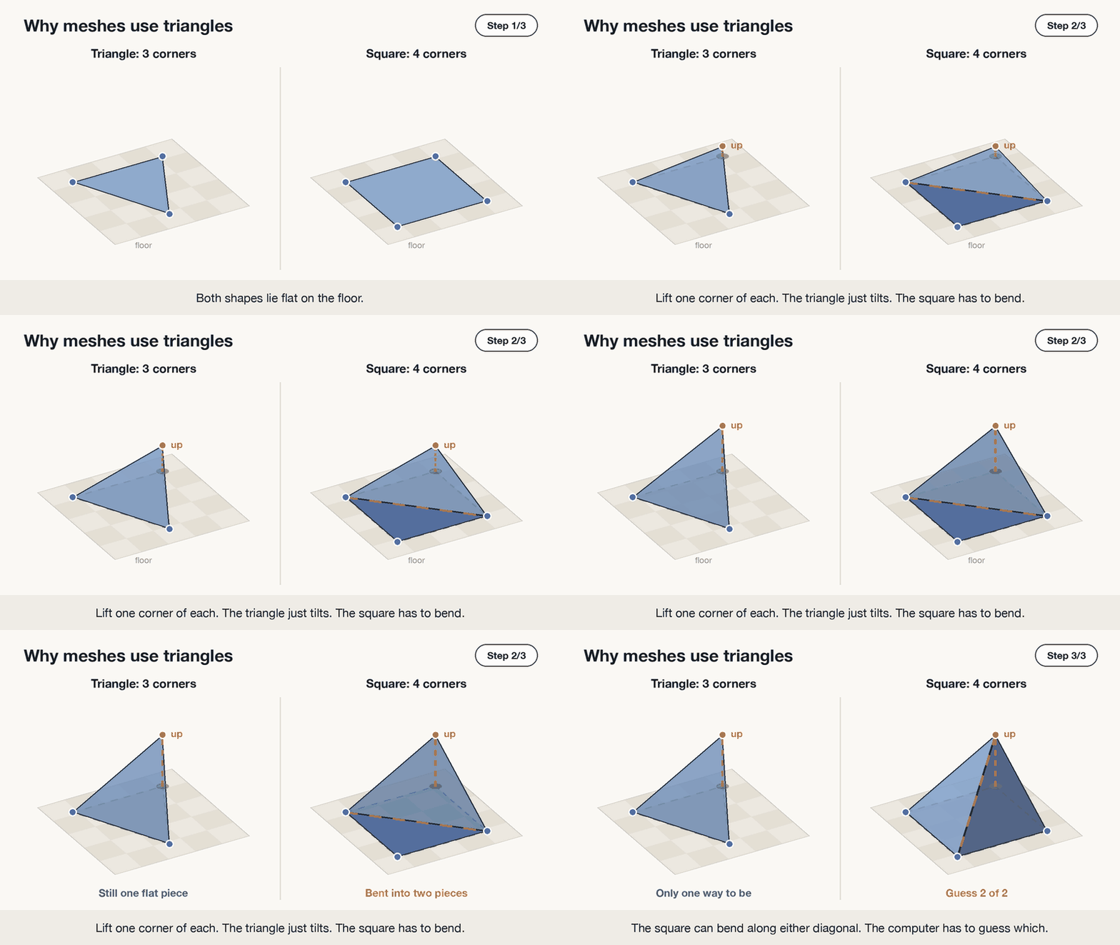Lift one corner: the triangle tilts but stays flat, the square has to bend, and there are two ways it could.

A triangle never needs that guess. That makes it easy to draw on screen, shade and measure, so games, 3D design tools and 3D printers all build their shapes out of triangles.

Reading a mesh file line by line

A real hill mesh has tens of thousands of triangles, which is too many to look at. So here’s the hill shrunk to the bare minimum: five points and four triangles, roughly a pyramid. On the right is how an OBJ file stores it. OBJ is plain text, so you could type this out in Notepad.

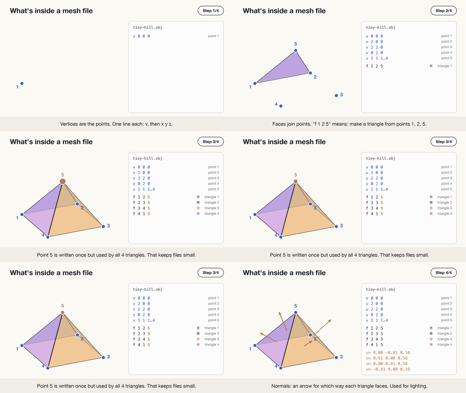An OBJ file is a list of points, followed by a list of triangles that refer back to them.

The v lines are the vertices, each with its x, y and z (the height). The f lines are the faces, and they hold no coordinates at all, only point numbers. f 1 2 5 reads as “a triangle using the 1st, 2nd and 5th points from the list above”.

Keeping the two lists separate saves a lot of space. The top of the pyramid is written once, yet all four triangles use it. In a full-size terrain mesh, a typical point sits at the corner of about six triangles, and it still only gets written down once.

The orange arrows are normals. Each one points straight out from the front of a triangle. Viewers use them for shading: faces turned toward the light come out bright, faces turned away come out dark. When a mesh shows up black or looks inside out, a flipped normal is nearly always the reason.

Files can carry more than this: a colour per point, or a photo wrapped over the surface (a texture), which is how drone models end up looking photographic. Strip those away and you’re back to the same two lists.

Two ways to join the dots

Choosing which points become triangles is the actual meshing step, and the right method depends on the shape you scanned.

Terrain allows a shortcut. Look down at the hill from directly above and ignore height for a moment. You’re left with a flat scatter of dots, and joining dots on a flat page is a solved problem. The standard method, Delaunay triangulation, prefers chunky, nearly even triangles over long thin ones. Once the flat net is made, give every point its height back and the net rises into the shape of the hill.

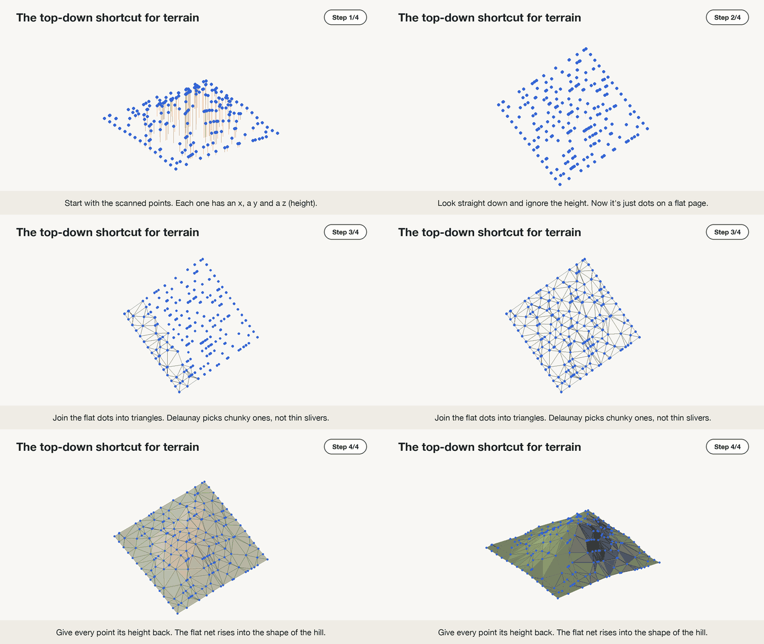Flatten, join the dots, lift back up.

The shortcut needs one height per spot on the map, which is true for open ground and false for almost anything built. Mapping people call a terrain mesh made this way a TIN (triangulated irregular network). It’s an ordinary mesh with a GIS name.

Buildings are where the shortcut breaks. Picture a house with a balcony and stand right under the balcony’s edge. From above, that’s one spot on the map. But the scanner caught three things there, stacked on top of each other: the top of the balcony, the underside of the balcony, and the ground below.

The shortcut only allows one height per spot. Given three, it has no idea which points belong together, so it joins them in a zig-zag, from balcony to ground and back again.

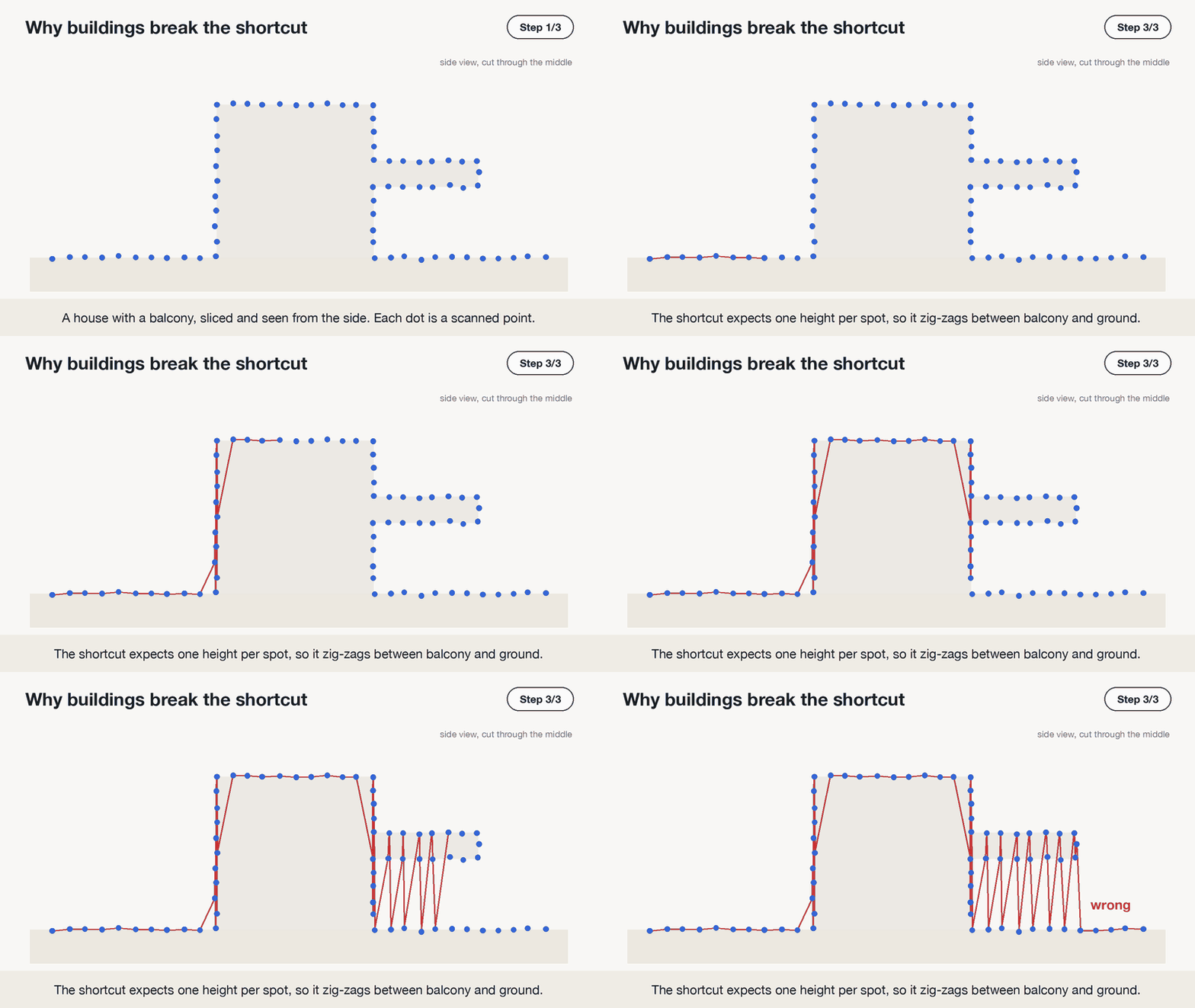A slice through the house. Under the balcony, the shortcut can’t tell what goes with what.

The same thing happens with bridges, statues, caves, trees, anything with an overhang. For these, the fix is to stop flattening. The points stay in 3D, and the mesh is built in two stages.

First, normals. Every point gets a short arrow pointing out of the surface, into the open air. The software works this out by looking at each point’s nearest neighbours: if they form a flat wall, the arrow points straight out from it. These arrows say which side is outside, which matters for the next stage. Libraries like Open3D do this for you.

Then, the surface. There are two popular ways to do it:

• Ball pivoting rolls an imaginary ball along the outside of the points, the side the arrows point to. Whenever the ball rests on three points at once, they become a triangle. It follows the real shape closely, sharp corners included. The catch is that where points are too far apart, the ball falls through and leaves a hole.
• Poisson reconstruction wraps one smooth skin over all the points at once, a bit like shrink-wrap. It never leaves holes, but it rounds off sharp corners a little.

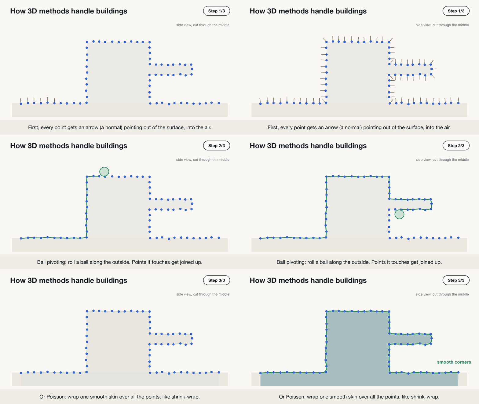Arrows first, then the surface: ball pivoting keeps sharp corners, Poisson gives a smooth skin.

Picking a file format

Four formats cover almost everything you’ll run into:

Format	What it is	Good for	Stores colour?
OBJ	Plain text, the v and f lines from above	Sharing with almost any 3D tool	Through a side file (.mtl) and a texture image
PLY	Like OBJ but usually binary, so smaller and faster	Scans and research tools like CloudCompare and MeshLab	Yes, per point
STL	Just triangles, no shared points	3D printing	No
glTF / GLB	Modern format made for the web and apps. GLB is the single-file version	Web viewers, AR, games	Yes, plus textures

Two more show up now and then. FBX is common in game and animation tools. 3D Tiles is for scans the size of a city: the mesh is split into chunks so a browser only downloads the part you’re looking at.

LAS and LAZ aren’t on the list because they aren’t mesh formats. They hold points only, which is exactly why Blender turned the scan away at the start.

Format choice affects file size more than you might expect. These are all the same real hilltop from later in this post (62,017 points, 124,001 triangles), saved four ways:

File	Size
tabor.glb	2.1 MB
tabor.ply	2.2 MB
tabor.obj	4.6 MB
tabor.stl	5.9 MB

OBJ pays for being readable: 173.94000000 is 12 characters of text where a binary format spends 4 bytes. STL is the largest because it throws away the shared-points trick and writes all three corners of every triangle in full, so each point appears about six times.

Build one from a scan

Setup: Python 3.11 or newer, plus uv.

For data, grab the scan I used (3.8 MB). It’s a real one: a 200 × 200 m square around the top of Mount Tabor, a small wooded hill in Portland, Oregon. It comes from a 2019 aerial survey by the US Geological Survey (USGS), which is public domain, so anyone can use it. It holds 549,120 points: ground, trees and some noise. With this file, your output will match the numbers below exactly.

When you want other places, OpenTopography and the USGS LiDAR Explorer both offer free downloads. Start with a small area, since real files run into gigabytes quickly.

Create a project with four packages:

uv init tabor-mesh
cd tabor-mesh
uv add "laspy[lazrs]" scipy trimesh fast-simplification

laspy reads LiDAR files, and the [lazrs] part lets it open compressed .laz files too. scipy provides Delaunay, trimesh holds the mesh and writes every format, and fast-simplification is used near the end to shrink it.

Drop tabor.laz into the folder and save this as tabor_to_mesh.py:

import laspy
import numpy as np
import trimesh
from scipy.spatial import Delaunay

# Read the LiDAR file
las = laspy.read("tabor.laz")

# Keep only ground points (class 2), so trees and buildings are left out
ground = las.points[las.classification == 2]

# Put the coordinates into one table: one row per point, columns x, y, z
points = np.column_stack([ground.x, ground.y, ground.z])

# Move everything close to zero so no precision is lost when saving
offset = points.min(axis=0)
points = points - offset

# The top-down shortcut: join the points into triangles using only x and y
triangles = Delaunay(points[:, :2]).simplices

# Put the 3D points (with height) and the triangles together into a mesh
mesh = trimesh.Trimesh(vertices=points, faces=triangles)
print(mesh)
print("surface area:", round(mesh.area), "m²")

# Save the same mesh in four formats; the file ending picks the format
mesh.export("tabor.obj")
mesh.export("tabor.ply")
mesh.export("tabor.stl")
mesh.export("tabor.glb")

# Make a lighter copy with about 2,000 triangles and save it too
small = mesh.simplify_quadric_decimation(face_count=2000)
small.export("tabor_small.glb")
print(small)

Then:

uv run tabor_to_mesh.py

Output:

<trimesh.Trimesh(vertices.shape=(62017, 3), faces.shape=(124001, 3))>
surface area: 42942 m²
<trimesh.Trimesh(vertices.shape=(1014, 3), faces.shape=(2000, 3))>

Out of 549,120 points, 62,017 were ground. Those became 124,001 triangles.

There’s the measurement a point cloud couldn’t give us. The square is 200 × 200 m, so 40,000 m² seen from above, but the actual surface of the hilltop is about 42,942 m². The slopes add roughly 7%.

A few lines are doing more than they look:

las.classification == 2 throws away everything except ground. Every point in a LAS file carries a label: 2 means ground, 3 to 5 are low to high vegetation, 6 is buildings, 7 and 18 are noise. Not every survey uses every label. This one marked the ground and the noise and left the trees as 1, “unclassified”. Either way, keeping only class 2 leaves just the bare earth.

Delaunay(points[:, :2]) is the top-down shortcut. The [:, :2] keeps only x and y, so the triangles are chosen as if the hill were flat. The next line pairs those triangles with the full 3D points, which lifts the net back up.

points - offset looks like housekeeping, but leave it out and the mesh breaks:

Real LiDAR uses map coordinates in metres. In this file, the y values are around 5,039,900. GLB and STL store numbers with roughly 7 significant digits, and at that size the smallest step they can represent is half a metre. The hill comes out as a staircase. Shifting everything close to zero first avoids that. Hold on to offset if the mesh ever needs to go back onto a map.

Seeing the result

Drag tabor.glb onto gltf-viewer.donmccurdy.com for the quickest look. It runs in your browser and doesn’t upload the file anywhere. MeshLab, CloudCompare and Blender are free and open any of the four files.

Also worth doing once: open tabor.obj in a text editor and scroll. It’s the same v and f lines as the pyramid, about 186,000 of them.

Making it lighter

The last two lines of the script exist because scan meshes are far heavier than they need to be. A flat field described by thousands of tiny triangles looks identical to the same field described by a handful of big ones.

Reducing triangles while holding the shape is decimation. It merges triangles on flat ground and keeps them dense where the surface curves.

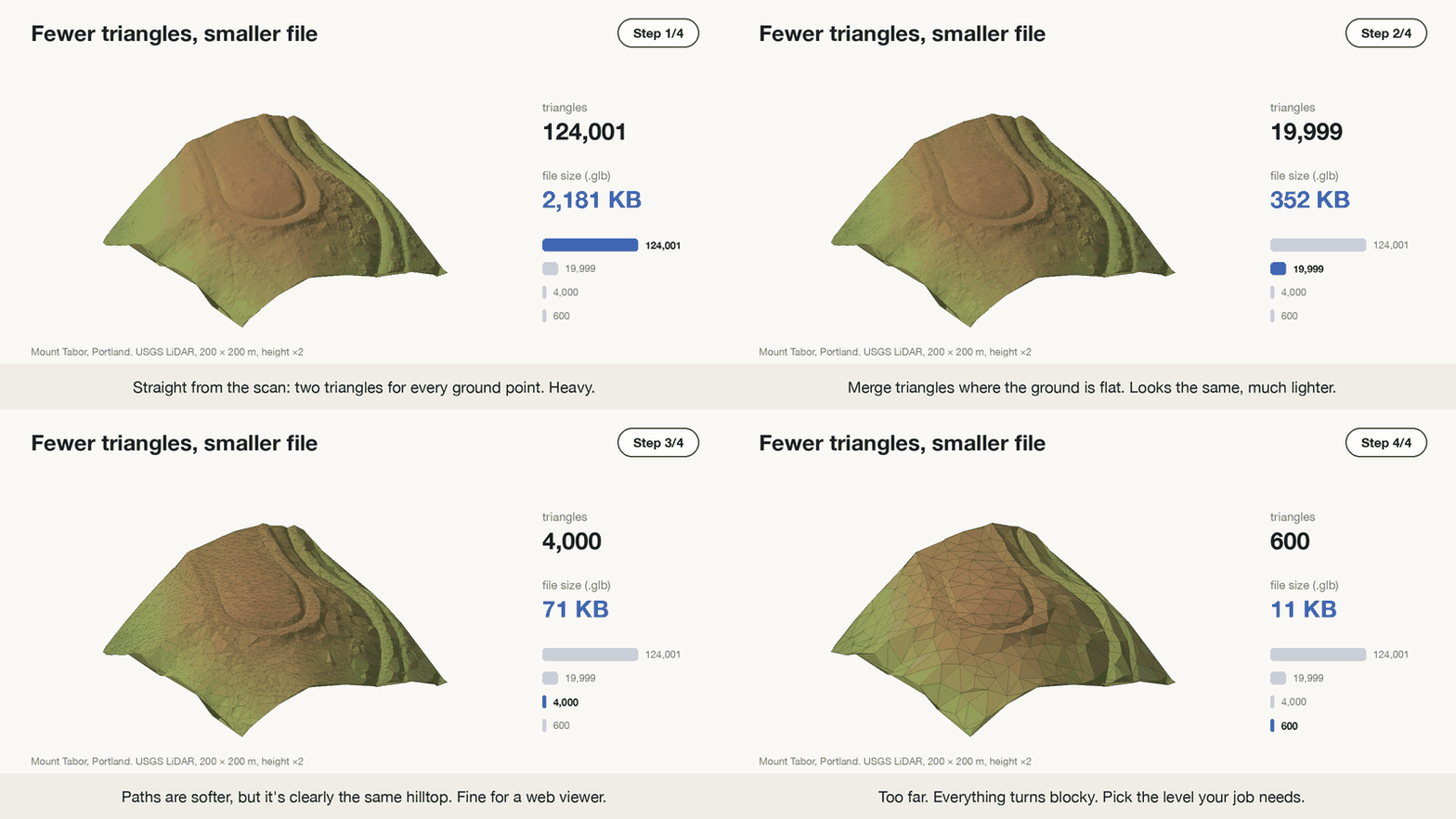The file shrinks much faster than the hill changes.

At 20,000 triangles the file is a sixth of the size and looks the same. At 4,000 the paths on the hilltop get softer, but it’s clearly the same place. At 600 everything turns blocky. The right stopping point depends on the job: volume calculations for a quarry need detail, a hill in the background of a game doesn’t.

Anything going on a website should be decimated. One hilltop at 2 MB is fine. A whole town at that density would be gigabytes.

When the mesh looks wrong

Long stretched triangles or flat patches. These mark gaps in the scan. LiDAR doesn’t reach under parked cars or into thick bushes, and water barely reflects the laser at all. Delaunay doesn’t know about gaps, so it bridges them with long slivers.

Needles sticking up (or down). A bird, a power line or some dust gives a stray point well above the ground, and the mesh dutifully pulls a spike up to meet it. A bad reflection can do the same thing below the ground. Keeping only class 2 clears most of them. CloudCompare’s outlier filter handles the rest.

A lumpy blanket instead of a hill. That’s what you get if trees are left in. Skip the classification filter on a forested scan and the mesh drapes over the canopy. That has its uses (it’s called a surface model), but it isn’t terrain.

Black or inside-out faces. Normals are pointing the wrong way. Most viewers have a flip-normals option, and trimesh has mesh.fix_normals().

Do you even need a mesh?

Not always. A rough guide:

• Keep the point cloud when the original measurements matter, like checking scan quality or classifying trees. Every mesh is a simplification of it.
• Use a height map (a raster, or DEM) for GIS jobs like contours and flood modelling. It’s a grid where each cell holds a height, quick to work with, but it can’t describe a wall or an overhang.
• Build a mesh when you need an actual surface: printing, games, web viewers, area and volume, or anything seen from more than one side.

The hill would work as any of the three. A temple with carved pillars only works as points or a mesh.

One last experiment with the same file: delete the classification == 2 line, so every point goes in, and run the script again. Then open both meshes side by side.

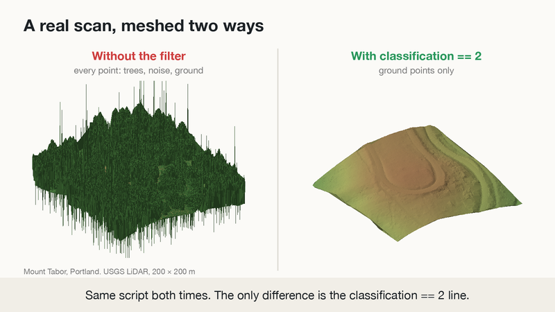Same scan, same script. On the left, every point. On the right, ground only.

On the left, the mesh drapes over the treetops, and the noise points pull out thin spikes above and below. On the right is the ground underneath: the hilltop, the loop road around it and the paths down the slope, all hidden under the trees until the filter took them away.

The surface area tells the same story. With the filter it’s 42,942 m². Without it, the script reports 1,465,173 m², about 34 times bigger, because every spike and every bump in the treetops adds surface. One line of code makes all that difference.

Further reading

• laspy documentation
• trimesh documentation
• LAS specification, including the point classes
• glTF overview from Khronos
• OpenTopography (free LiDAR data)
• USGS LiDAR Explorer
• CloudCompare and MeshLab